Basics of data visualization for behavioral scientists
Session 1 Basics of data wrangling in R
1.1 Installing R and RStudio
We will start by installing R – which is the programming language we will be using to learn how to visualize data – as well as RStudio – which is an integrated development environment for R. In case you’re not sure what the difference between one thing and the other is, think of R as the actual computer or engine behind all the calculations and operations you will be performing, while RStudio is the beautiful and very helpful interface that makes it all much more enjoyable and streamlined as a programming/ analysis experience.
To install R, go to the following webpage > https://cloud.r-project.org/ < and select your operating system as well as your R version. As the page will tell you, you want to go for base R if this is your first install. Once you’ve installed R, open it and let’s get familiarized with some basic concepts and operations, as well as with the way R syntax generally works.
R serves first and foremost as a computing tool, that is, as a tool for calculating things. To get started, type in your R console 2 + 2, as shown in the code box below, and see what happens. To run the code in R, either press Enter or select the bit of code and press Ctrl + Enter. Below the inputted code you should see the result of your operation, which in this case is straightforward and not in any sense unexpected.
2 + 2## [1] 4In R you are able to perform the same arithmetic operations you’d be able to perform in any programming language, such as subtraction 2 - 2, multiplication 2 * 2, or division 2 / 2. You are also able to use logical operators to check whether a given relation between two or more elements is true or false. Suppose you want to know whether 2 is larger than 3, you can check that by running the code below.
2 > 3## [1] FALSEUnsurprisingly, the output of the code above tells us that 2 is not greater than 3. Other important logical operations include checking whether two elements are equal to one another 2 == 3, not equal to another 2 != 3, or whether the relation between multiple sets of elements or multiple individual operations is true or false. For instance, notice the difference between the output of the two code snippets below.
2 >= 3 | 3 >= 3## [1] TRUE2 >= 3 & 3 >= 3## [1] FALSEWhile in the first case the output of the joint logical operation is true, in the second case it is false, and this has to do with the usage of the operators | and &. What these operators do is to evaluate different combinations of individual outputs. In both cases, the individual operations which get evaluated consist of checking whether a given value is equal to or higher than 3. | indicates that the output of either one or the other individual operation should be equal to or greater than 3, while & indicates that the output of both individual operations should be equal to or greater than 3. These sorts of logical operations will come in very handy later when we manipulate data structures consisting of lists of several values.
Now, other than performing basic operations such as the ones above, more importantly for our purposes we will use R to manipulate and organize data in ways which help us discover and highlight patterns which we deem interesting as data analysts. More than that, we will use R to create visual representations of data so as to help us communicate any interesting data patterns to an external audience. In this course, we will learn how to communicate data to an audience which is academic or to some extent or another familiar with the goals and interests of scientific communication. But first let’s learn some more about the basics in R.
This is a good point to bring in RStudio, which will only enhance our experience as R data analysts. You can download RStudio here > https://rstudio.com/products/rstudio/download/. Note that you need to have base R installed to be able to run RStudio. Once you’ve installed RStudio, let’s have a look at the interface it offers us.
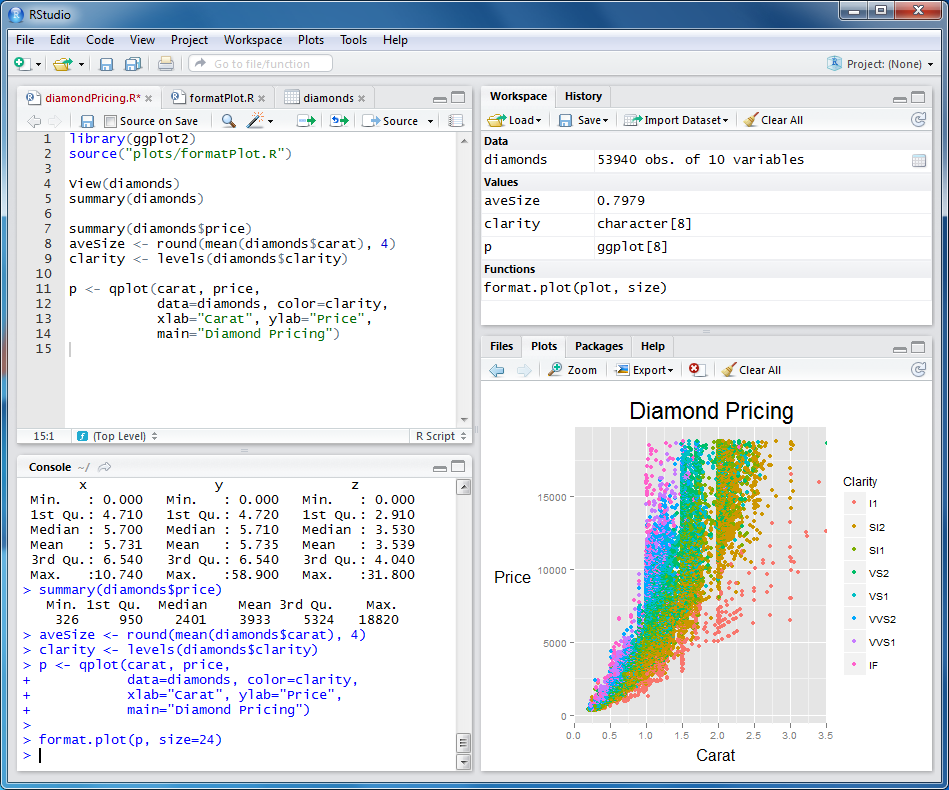
RStudio interface
In a nutshell, RStudio has 4 panels or regions of interest, as shown in the picture above. At the top left you have the region where you will usually have an R script, which is the document in which you type and record your R commands, the bits of code that will generate an output after the R engine has done its magic. This panel need not necessarily house a plain code script, as we will see it can also contain a document which gets converted into a reader-friendly file, such as a PDF or an HTML. But that’s where you will type things and organize the logic of your analyses/ programs. Right below that is the RStudio console, which, much like the console in base R, showcases the output of whatever chunks of code you run. Any time you ask R to output some data summary or to run an operation this is where you will see it, usually in a condensed format given the running window character of the panel. Use the console to inspect what your code does but do not type your commands straight into it as the console will not save anything that is displayed in it. At the bottom right you have a multi-purpose panel which is usually used to view any graphical representations of your data, your plots, but also to view and locate any files or to read the always-handy entries from the different sources of R documentation. Last, at the top right you will find a panel where you can see any data structures you create or load during your R sessions, including data sets, R variables, temporary functions and shortcuts you create and much more. This is where most of your data management will occur, so eventually you will learn to keep your environment minimally clean and tidy.
1.2 Creating data structures
Now that we know where to write code in RStudio and where to look for the output and representation of our operations, let’s have a look at how we can create and manipulate different types of data in R. Let’s bring back our basic arithmetic operation from above, 2 + 2. It’s fine simply running the operation as this chunk of code currently does, but usually you will want to access the output of one operation and feed it to another operation, or maybe you will want to store it locally for purposes of record-keeping and data management. Let’s then store the result of 2 + 2 in a new variable, which we can call op1, short for operation one. You can do that in R by assigning an operation or an already existing code output to a label, an unique identifier which stands for your newly created variable. Simply type the name of your new variable followed by an arrow and the operation or code output you wish to assign to it.
op1 <- 2 + 2Now, in order to check if the assignment was sucessful, you can try calling your new variable. Type in op1 and run the code to see what happens. You should see the result of the operation 2 + 2, which is what you stored under the label op1. Notice that calling op1 only shows the actual output of the operation, and not the source of that output. This is an important aspect of variable assignment.
op1## [1] 4Before we move on to more interesting cases of data manipulation, let’s have a look at what happens if you try to manipulate the variable you created. There’s two things we can do here. We can use op1 in a new operation without modifying the variable itself, which works by using the value associated with op1 without changing its representation:
op1 + 2## [1] 6Alternatively, we can store the result of our manipulation of op1 in a new variable, which we can call op2. Now we have two variables which we can manipulate and call back whenever we want. Notice how those two variables are now visible in your environment panel on the right, which means that they are retrievable within your current R session. If you wish to store your progress for future work, however, you should save an R script with the code used to create op1 and op2. When you open that script in a future R session and run the respective code, the variables will be created anew and will become visible in your environment panel.
op2 <- op1 + 2

op2
## [1] 6As you can imagine, storing the output of simple operations like the one above might not be that useful in itself. Usually, you will want to manipulate more complex variables consisting of lists of several elements, for instance several numbers or tokens of a given category. Let’s create a list of numbers and do some more basic calculations with it. To create a list of elements, called a vector in R, you can use the command c() as shown below:
numbers <- c(2, 3, 5, 9)

numbers
## [1] 2 3 5 9As per usual, calling your variable shows the elements stored in it. In our toy example, this is a vector with four numbers. You can inspect any R object, whether a single variable or more complex data structures as we will construct later, by using the function str(). Try that yourself and see what it tells you about the vector numbers.
str(numbers)## num [1:4] 2 3 5 9str() is useful in two ways: first, it tells you what type of an object your variable is. This is something that you will usually know if you create the variable yourself – in fact, it is something that you should know, as it will make your life easier later on – but in case you don’t know or can’t remember, str() is a good method of finding it out. Then, str() will also show you the length of your object, in this case a vector of length 4, i.e. a vector composed of 4 elements.
Let’s turn our focus to object types. In the case of numbers, str() diagnoses the vector as being numeric, which of course means that it is composed of numbers. But numeric is not the only vector type in R, there is in fact a number of other vector types, all of which are primitive data structures in R, which is to say that they act as building blocks for more complex data structures. The most important primitives for us are:
Logical vectors, which contain elements that are marked as either true or false, most likely stored as the output of some logical operation or as a reference to a binary category (
lv <- c(TRUE, FALSE, FALSE, TRUE));Numeric vectors, which contain elements that are numbers, including numbers with decimals (
nv <- c(10, 15.6, 4, 7.9));Integer vectors, which contain elements that are whole numbers (
iv <- c(7, 15, 2, 57));Character vectors, which contain elements that are strings of text, including orthographic representations of numbers and Arabic numerals without the underlying number representation in R (
cv <- c("butterfly", "5", "four", "false")).
One important and useful characteristic of vectors in R is that they can be converted into a nominal variable regardless of the actual vector type. Factors as they are called in R are vectors that have labels associated with each unique element stored in them. This might not seem particularly useful at this point, but it will be when we start dealing with meaningful data. For now let’s just remember that a factor consists of a mapping between nominal values, which are arbitrary labels, and a set of elements. Notice that there might be more elements than unique labels, depending on the number of repeated elements. The code below converts numbers into a factor and checks the structure of the converted vector.
numbers <- as.factor(numbers)

str(numbers)
## Factor w/ 4 levels "2","3","5","9": 1 2 3 4Vectors can be combined to create larger R objects. If multiple vectors of the same type are combined, the result is a matrix, a two-dimensional data structure with multiple rows and columns. If multiple vectors of different types are combined, the result is a data frame, which is also a two-dimensional data structure. Another useful type of data structure is an array, which is similar to a matrix, i.e. it consists of a single element type, but can have an n number of dimensions. The code below creates a new vector composed of letters, a character vector called letters. When you create a character vector, you need to use quotation marks to demarcate each individual element, as shown below. We then check the structure of the newly created vector in order to make sure that the object type is correct. Finally, we combine numbers and letters into a data frame which we call df1, and use str() to get some more details about the newly created data frame.
letters <- c("a", "f", "m", "t")

str(letters)
## chr [1:4] "a" "f" "m" "t"df1 <- data.frame(numbers, letters)
str(df1)## 'data.frame': 4 obs. of 2 variables:
## $ numbers: Factor w/ 4 levels "2","3","5","9": 1 2 3 4
## $ letters: Factor w/ 4 levels "a","f","m","t": 1 2 3 4By inspecting our new data frame we can see that letters, originally a character vector, is now a factor, each individual letter consisting of a label, or as R calls it, a level, of its own. There is an explanation for this: when creating a data frame R converts character vectors to factors by default. This can lead to confusion later on when you manipulate your variable, now part of a data frame. In case the automatic conversion is unintended, you can avoid it by specifying the argument stringsAsFactors in the data.frame() function.
NOTE: Starting with R version 4.0, released in June 2020, data.frame() does not convert character vectors to factors by default anymore. If you have installed R from scratch right before working on this session, you will be using R version 4.0 or newer, which means your default is stringsAsFactors = FALSE.
Functions in R, like data.frame(), have arguments, which are slots that get filled with both mandatory and optional information. Think of arguments as switches that can be manipulated in order to produce slightly different outputs with the same function call. In the code below, we change stringAsFactors from its default TRUE to FALSE in order to avoid the conversion of our character vector. Notice the difference in the output.
df1 <- data.frame(numbers, letters, stringsAsFactors = FALSE)

str(df1)
## 'data.frame': 4 obs. of 2 variables:
## $ numbers: Factor w/ 4 levels "2","3","5","9": 1 2 3 4
## $ letters: chr "a" "f" "m" "t"1.3 Subsetting and manipulating data
Having created our toy data frame df1 let’s play around with it for a little while. Let’s start by calling our data frame, this time without using the usual str() command. Given that df1 is a minuscule data set, it should be no problem visualizing it straight in the console. Alternatively, you could click on the data frame object in your environment panel to have a full view of the data, which should come in handy when we deal with larger data sets with dozens or hundreds of rows/ columns.
df1## numbers letters
## 1 2 a
## 2 3 f
## 3 5 m
## 4 9 tAs you can see, our two variables, numbers and letters, are organized as columns in the data frame, with the individual values organized vertically bellow their respective variable names. You have probably noticed this before, but data frames have a tabular format, which is only possible given that each of our variables has the exact same number of elements or values. Now suppose we want to add more information to our data set, suppose we want to record whether the values associated with our two existing variables are presented in the right order, numbers in ascending order and letters in alphabetical order. We can start by creating a variable called order_numb, which indicates whether the number value of a given observation is given in the correct ascending order. Let’s then merge that with df1 and save the resulting data frame with the same name, df1.
order_numb <- c(TRUE, TRUE, TRUE, TRUE)

df1 <- data.frame(df1, order_numb)

df1
## numbers letters order_numb
## 1 2 a TRUE
## 2 3 f TRUE
## 3 5 m TRUE
## 4 9 t TRUENow let’s create a fourth variable called order_let, which indicates whether the letter value of a given observation is given in the correct alphabetical order. This time, however, let’s use an alternative to merging the vector and the data frame together, which is what data.frame() does, and so let’s add the vector order_let straight to the already existing df1 data frame. Notice the usage of the operator $.
order_let <- c(TRUE, TRUE, TRUE, TRUE)

df1$order_let <- order_let

df1
## numbers letters order_numb order_let
## 1 2 a TRUE TRUE
## 2 3 f TRUE TRUE
## 3 5 m TRUE TRUE
## 4 9 t TRUE TRUEWe now have order_numb and order_let, two logical vectors, indicating whether the number and letter values of a given observation are ordered properly. However, if we think about it, these two variables are in a sense instances of the same superordinate variable, something we could call order. This is a very good moment to introduce the concept of tidy data, which will be very important for us as we get our hands on real data. The picture below illustrates what tidy data looks like.
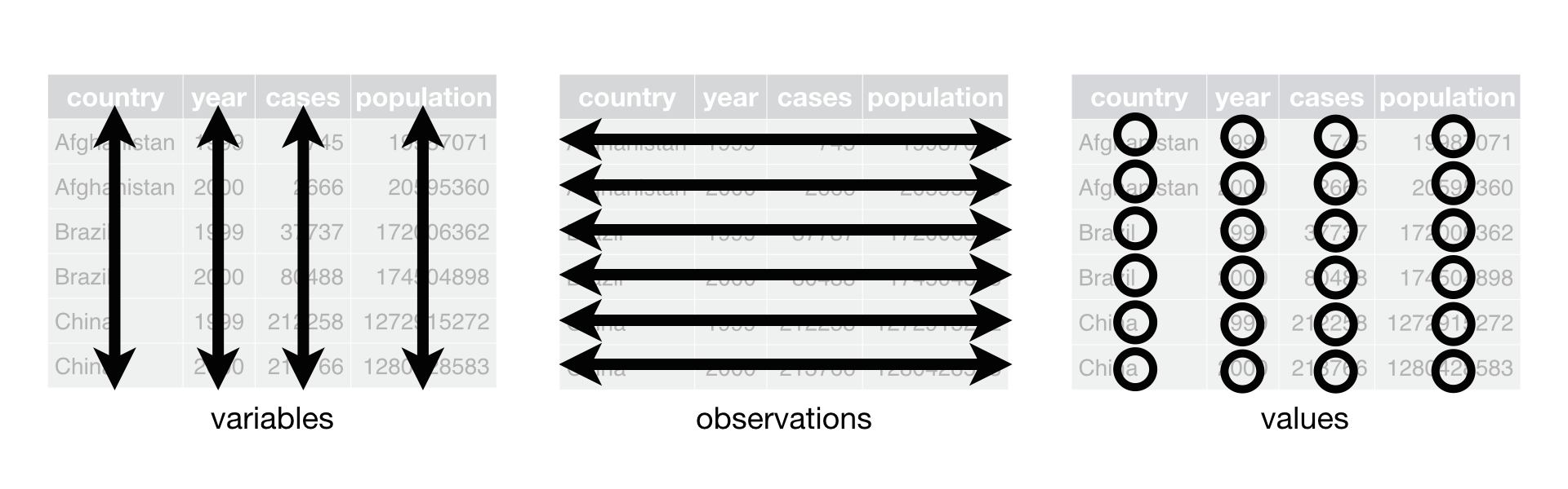
Tidy data
As we can see, aside from each row reflecting an individual observation and each cell consisting of an individual value, in a tidy data set the columns relate to individual variables. That is not really the case in df1, if we consider that order_numb and order_let both relate to the same variable. Let’s then change how our data frame is organized. For that, we will need special tools, which we will borrow from a very handy R toolkit known as the tidyverse. The tidyverse is a collection of packages – small extensions to base R which feature extended or improved function(alities)s – which greatly improve the tasks of everyday data analysis. Some of its packages, including dplyr, tidyr, and ggplot2, will be the bread and butter of practically any data analytic endeavor in R. To install the tidyverse, call install.packages("tidyverse").
Once installed, any R package can be loaded by calling library(). Packages need only be installed once, however, each new session they need to be loaded anew if to be used in that session. A best practice in R programming is to load any necessary packages right at the beginning of an R session/ script, before they are actually needed later in the body of the script. For now, we will need the function pivot_longer() from the tidyr package, but we will load the tidyverse as a whole, which will prevent us from having to load other individual tidyverse packages later. Let’s then use pivot_longer() to reshape our data frame, moving our two order_ variables and their respective values into a new arrangement that reflects the common basis between order_numb and order_let. pivot_longer() allows us to elongate our data set, increasing the number of rows and decreasing the number of columns. In this particular case, we end up with the same number of columns as we started, but had we had more than two order_ variables the resulting number of columns in df1_long would have been smaller than in df1.
library(tidyverse)## -- Attaching packages --------- tidyverse 1.3.0 --## v ggplot2 3.3.2 v purrr 0.3.4
## v tibble 3.0.3 v dplyr 1.0.2
## v tidyr 1.1.2 v stringr 1.4.0
## v readr 1.3.1 v forcats 0.5.0## -- Conflicts ------------ tidyverse_conflicts() --
## x dplyr::filter() masks stats::filter()
## x dplyr::lag() masks stats::lag()df1_long <- pivot_longer(df1, cols = starts_with("order"), names_to = "order", values_to = "correct")
df1_long## # A tibble: 8 x 4
## numbers letters order correct
## <fct> <chr> <chr> <lgl>
## 1 2 a order_numb TRUE
## 2 2 a order_let TRUE
## 3 3 f order_numb TRUE
## 4 3 f order_let TRUE
## 5 5 m order_numb TRUE
## 6 5 m order_let TRUE
## 7 9 t order_numb TRUE
## 8 9 t order_let TRUEAs you will notice as you start coding in R, usually there are multiple alternative ways of achieving the same desired end result. One alternative to our reshaping operation as coded above involves using the so-called pipe operator %>%, which is one of the many handy tools that come with the tidyverse. If we inspect our code, more specifically the arguments in the pivot_longer() function, we see that the original data frame, df1, is called inside the function as its first argument. What that means is that pivot_longer needs to know which data frame is to be reshaped, the specific instructions of how exactly to reshape it being given in the arguments names_to and values_to. Now, in many functions you will need to specify which data source is the object of whatever operation the function is supposed to perform. If you are performing a single operation at a time, specifying the data source in the function argument is fine, however, if you are to perform several distinct operations, all sharing the same data source, chaining those operations might be a more convenient way of doing things. This is where the pipe operator comes in. Using %>% to ‘pipe’ a data source into one or more operations is a great way of saving yourself typing and writing a more fluid, though arguably less explicit, chunk of code. Run the code below and check whether the output differs from the code chunk above.
df1_long <- df1 %>%
  pivot_longer(cols = starts_with("order"), names_to = "order", values_to = "correct")

df1_long
## # A tibble: 8 x 4
## numbers letters order correct
## <fct> <chr> <chr> <lgl>
## 1 2 a order_numb TRUE
## 2 2 a order_let TRUE
## 3 3 f order_numb TRUE
## 4 3 f order_let TRUE
## 5 5 m order_numb TRUE
## 6 5 m order_let TRUE
## 7 9 t order_numb TRUE
## 8 9 t order_let TRUENow let’s learn how to subset our data frame. Depending on what it is we want to do, we might want to extract a whole variable, a certain number of observations, or a single data value. Suppose we want to inspect the numbers variable without calling the whole data frame. We can that do by using either of the options below.
df1_long$numbers## [1] 2 2 3 3 5 5 9 9
## Levels: 2 3 5 9df1_long[, 1]## # A tibble: 8 x 1
## numbers
## <fct>
## 1 2
## 2 2
## 3 3
## 4 3
## 5 5
## 6 5
## 7 9
## 8 9Note how the subsetted values are the same, though the output is presented in a slightly different way. In the first case we resorted to the $ operator, which we had used before already to add a variable to our data frame. Here, the $ operator is used to single out an individual variable from the data frame. In the second case we resorted to squared brackets [,], which are used to specify which rows and columns from our data frame, a tabular data structure, we want to extract. The 1 after the comma stands for the column: that tells R to extract the 1st column, i.e. the numbers column, from df1_long. Notice how before the comma nothing is specified: that tells R to extract all rows from the data frame. An alternative to that would be to explicitly specify rows 1 to 8 df1_long[1:8, 1], which would result in all 8 rows being extracted, exactly the same result as above.
Now, suppose you only want to extract the first two rows of numbers. For that, we would specify our rows [1:2, x] and then our column [x, 1].
df1_long[1:2, 1]## # A tibble: 2 x 1
## numbers
## <fct>
## 1 2
## 2 2What if we only want to extract a single value from df1_long? For that, we should specify the precise coordinates of that value, say 1st column and 4th row [4, 1].
df1_long[4, 1]## # A tibble: 1 x 1
## numbers
## <fct>
## 1 3These are all the basic ways of extracting bits of data from a data table in R. In fact, these are the base R ways of doing it. But we also have the tidyverse tools at our disposal, which make some of these operations more streamlined. Let’s repeat the same operations from the code chunks above but now using functions from the dplyr package. First, let’s extract the numbers variable from df1_long, incorporating the %>% operator as well. Notice how you can do that by either specifying the column number or the column name.
df1_long %>%
  select(1)
## # A tibble: 8 x 1
## numbers
## <fct>
## 1 2
## 2 2
## 3 3
## 4 3
## 5 5
## 6 5
## 7 9
## 8 9df1_long %>%
select(numbers)## # A tibble: 8 x 1
## numbers
## <fct>
## 1 2
## 2 2
## 3 3
## 4 3
## 5 5
## 6 5
## 7 9
## 8 9You can, of course, also select more than a single variable at a time. Suppose we wanted to extract both numbers and letters. For that we could use either of the options below.
df1_long %>%
  select(1:2)
## # A tibble: 8 x 2
## numbers letters
## <fct> <chr>
## 1 2 a
## 2 2 a
## 3 3 f
## 4 3 f
## 5 5 m
## 6 5 m
## 7 9 t
## 8 9 tdf1_long %>%
select(numbers, letters)## # A tibble: 8 x 2
## numbers letters
## <fct> <chr>
## 1 2 a
## 2 2 a
## 3 3 f
## 4 3 f
## 5 5 m
## 6 5 m
## 7 9 t
## 8 9 tNow let’s use a dplyr function to extract only values that meet a certain criterion. Say we want to extract only the observations that have a number value above 2. We can try the code below, using the filter() function.
df1_long %>%
  filter(numbers > 2)
## Warning in Ops.factor(numbers, 2): '>' not meaningful for factors## # A tibble: 0 x 4
## # ... with 4 variables: numbers <fct>, letters <chr>, order <chr>,
## # correct <lgl>This didn’t work the way we wanted, but luckily R throws error warnings to help us understand what might have gone awry. According to the warning, the greater-than operator > is not meaningful for factors. Let’s try to make sense of that. First, recall that the numbers variable is a factor, which means that the numbers are only stored as labels and not as actual numeric representations. Now the operation we are trying to perform only makes sense when applied to numeric or integer vectors, given that a nominal value cannot be greater than another nominal value. Let’s then try to convert numbers back to a numeric vector and attempt to perform the operation again.
as.numeric(df1_long$numbers)## [1] 1 1 2 2 3 3 4 4Even before we have the chance to try the extraction operation again, we can see that something went wrong with the factor conversion. The resulting vector does not seem to show the original numeric values but rather the labels associated with them in the factor representation. If we look for help in the documentation on factor, we find the following note:
as.numericapplied to a factor is meaningless, and may happen by implicit coercion. To transform a factor f to approximately its original numeric values,as.numeric(levels(f))[f]is recommended
Let’s then do what the R documentation recommends before we attempt to perform our original extraction operation again.
as.numeric(levels(df1_long$numbers))[df1_long$numbers]## [1] 2 2 3 3 5 5 9 9df1_long$numbers <- as.numeric(levels(df1_long$numbers))[df1_long$numbers]
df1_long %>%
filter(numbers > 2)## # A tibble: 6 x 4
## numbers letters order correct
## <dbl> <chr> <chr> <lgl>
## 1 3 f order_numb TRUE
## 2 3 f order_let TRUE
## 3 5 m order_numb TRUE
## 4 5 m order_let TRUE
## 5 9 t order_numb TRUE
## 6 9 t order_let TRUENow the factor conversion works seamlessly, and so does the subsequent extraction operation. Our failed attempts should serve as a reminder that one should always know what type of data they are trying to manipulate. In many cases, we won’t exactly know, for example, why a given operation won’t work on a vector of type factor or numeric. Such situations will usually require some research about the exact operator or function we’re trying to use, but overall knowing how our variables of interest are stored and represented in R is a must to any process of data manipulation and analysis. This will be particularly true when the data we deal with have meaningful counterparts in a study design, such as a group of participants or a particular type of measurement.
Let’s try one more trick before summarizing what we’ve learned so far. Currently, numbers is organized in an ascending order. But what if we wanted to display our number values in a descending order? We could create a new numbers vector with the reverse order, and then replace the old vector with the new one, but that is a pretty roundabout solution. Instead, we can use the dplyr function arrange(), as shown below.
df1_long %>%
  arrange(desc(numbers))
## # A tibble: 8 x 4
## numbers letters order correct
## <dbl> <chr> <chr> <lgl>
## 1 9 t order_numb TRUE
## 2 9 t order_let TRUE
## 3 5 m order_numb TRUE
## 4 5 m order_let TRUE
## 5 3 f order_numb TRUE
## 6 3 f order_let TRUE
## 7 2 a order_numb TRUE
## 8 2 a order_let TRUEThis seems to work just fine. Of course not always will we have a handy tidyverse function like arrange() to quickly solve our problems, but many recurring wrangling operations have been turned into functions to simplify data analysis in R. This is the exact reason why we use the tidyverse, as its packages make our job as data analysts much easier in many instances. This is not to say that one needs to rely on these packages and functions, in fact we can even create our own functions or use coding solutions that we might know from other programming languages. The point is to realize which options work best for our individual purposes, considering also the constrains of the data we have at hand.
In the next session of our course, before we learn how to plot data, we will talk about how to map data reflecting some of the measures typically found in behavioral research onto the data structures we can create and manipulate in R. For now, let’s recapitulate the key points that we learned in today’s session.
1.4 Session summary
In order to create a variable or assign something to an already existing variable we use the arrow operator
<-, e.g.op1 <- 2 + 2;In order to create a vector we can use the function
c(), wherec()contains the values or elements to be created, e.g.nv <- c(10, 15.6, 4, 7.9);In order to quickly gather information about a vector or any other data structure we can use the function
str(), e.g.str(nv);In order to convert any vector into a factor, which stores individual values as unique labels, we can use the function
as.factor(), e.g.as.factor(nv);In order to create a data frame, a tabular data structure made up of vectors of various types, we can use the function
data.frame(), e.g.data.frame(nv, cv);We learned that we should strive to keep our data tidy. In order to do that, we can perform several operations, such as elongating a data table with
pivot_longer, selecting and filtering variables withselect()andfilter(), or better arranging variables witharrange();Finally, we learned that we can feed a data source into one or more operations using the pipe operator
%>%, e.g.nv %>% filter( > 4).
1.5 Exercises
Convert df1_long back to its original, wide format. Try using the
pivot_wider()function from the tidyr package.Remove the variable letters from df1. Try using
select(), and for that inspect the function documentation using the Help tab on the lower right panel of RStudio.Find observations that have a numbers value above 4 and then add 4 to those values. Chain those two operations together using the pipe
%>%.Add a new variable to the data frame called order_both. This should be a logical vector that indicates whether both order_numb and order_let are true. If so, order_both should be
TRUE; if not, thenFALSE. Check the functionmutate()and use it to create the new variable.